Initialization Of Feedfoward Networks

Jefkine, 27 July 2016

Introduction

Weight initialization has widely been recognized as one of the most effective approaches in improving training speed of neural networks. Yam and Chow [1] worked on an algorithm for determining the optimal initial weights of feedfoward neural networks based on the Cauchy’s inequality and a linear algebraic method.

The proposed method aimed at ensuring that the outputs of neurons existed in the active region (i.e where the derivative of the activation function has a large value) while also increasing the rate of convergence. From the outputs of the last hidden layer and the given output patterns, the optimal values of the last layer of weights are evaluated by a least-squares method.

With the optimal initial weights determined, the initial error becomes substantially smaller and the number of iterations required to achieve the error criterion is significantly reduced.

Yam and Chow had previously worked on other methods with this method largely seen as an improvement on earlier proposed methods [2] and [3]. In [1] the rationale behind their proposed approach was to reduce the initial network error while preventing the network from getting stuck with the initial weights.

Weight Initialization Method

Consider a multilayer neural network with $L$ fully interconnected layers. Layer $l$ consists of $n_l+1$ neurons $(l = 1,2,\dotsm,L-1)$ in which the last neuron is a bias node with a constant output of $1$.

Notation

1. $l$ is the $l^{th}$ layer where $l=1$ is the first layer and $l=L$ is the last layer.
2. $o_{i,j}^l$ is the output vector at layer $l$ $$ \begin{align} o_{i,j}^{l} &= \sum_{i =1}^{n_l+1} w_{i\rightarrow j}^l a_{p,i}^l \end{align} $$
3. $w_{i\rightarrow j}^l$ is the weight vector connecting neuron $i$ of layer $l$ with neuron $j$ of layer $l+1$.
4. $a^l$ is the activated output vector for a hidden layer $l$. $$ \begin{align} a_{p,j}^{l} &= f(o_{p,j}^{l-1}) \end{align} $$
5. $f(x)$ is the activation function. A sigmoid function with the range of between $0$ and $1$ is used as the activation function. $$ \begin{align} f(x) = \frac{1}{1 + e^{(-x)}} \end{align} $$
6. $P$ is the total number of patterns for network training.
7. $X^1$ where $l=1$ is the matrix of all given inputs with dimensions $P$ rows and $n_l + 1$ columns. All the last entries of the matrix $X^1$ are a constant $1$.
8. $W^l$ is the weight matrix between layers $l$ and $l+1$.
9. $A^L$ is the matrix representing all entries of the last output layer $L$ given by $$ \begin{align} a_{p,j}^L &= f(o_{p,j}^{L-1}) \end{align} $$
10. $T$ is the matrix of all the targets with dimensions $P$ rows and $n_L$ columns.

The output of all hidden layers and the output layer are obtained by propagating the training patterns through the network.

Learning will then be achieved by adjusting the weights such that $A^L$ is as close as possible or equals to $T$.

In the classical back-propagation algorithm, the weights are changed according to the gradient descent direction of an error surface $E$ (taken on the output units over all the $P$ patterns) using the following formula: $$ \begin{align} E_p &= \sum_{p =1}^P \left( \frac{1}{2} \sum_{j}^{n_L}\left(t_{p,j} - a_{p,j}\right)^2 \right) \end{align} $$

Hence, the error gradient of the weight matrix $w_{i\rightarrow j}$ is:

$$\begin{align} \frac{\partial E_p}{\partial w_{i\rightarrow j}^l} &= \frac{\partial E_p}{\partial o_{i,j}^{l}} \frac{\partial o_{i,j}^{l}}{\partial w_{i\rightarrow j}^l} \\ &= \delta^{l}_{p,j} \frac{\partial}{\partial w_{i\rightarrow j}^{l}} w_{i\rightarrow j}^{l} a_{p,i}^{l} \\ &= \delta^{l}_{p,j} a_{p,i}^{l} \end{align}$$

If the standard sigmoid function with a range between 0 and 1 is used, the rule of changing the weights cane be shown to be: $$ \begin{align} \Delta w_{i,j}^l =&\ -\frac{\eta}{P} \sum_{p =1}^P \delta_{p,j}^{l}a_{p,i}^{l} \end{align} $$ where $\eta$ is the learning rate (or rate of gradient descent)

The error gradient of the input vector at a layer $l$ is defined as $$ \begin{align} \delta_{p,j}^l = \frac{\partial E_p}{\partial o_{p,j}^l} \end{align} $$

The error gradient of the input vector at the last layer $l = L - 1$ is

$$\begin{align} \delta_{p,j}^{L-1} &= \frac{\partial E_p}{\partial o_{p,j}^{L-1}} \\ &= \frac{\partial}{\partial o_{p,j}^{L-1}} \frac{1}{2}(t_{p,j} - a_{p,j}^L)^2 \\ &= \left( \frac{\partial}{\partial a_{p,j}^{L}} \frac{1}{2}(t_{p,j} - a_{p,j}^L)^2 \right) \frac{\partial a_{p,j}^{L}}{\partial o_{p,j}^{L-1}} \\ &= (t_{p,j} - a_{p,j}^L) \frac{\partial f(o_{p,j}^{L-1})}{\partial o_{p,j}^{L-1}} \\ &= (t_{p,j} - a_{p,j}^L) f'(o_{p,j}^{L-1}) \tag 1 \end{align}$$

Derivative of a sigmoid $f'(o^{L-1}) = f(o^{L-1})(1 - f(o^{L-1}))$. This result can be substituted in equation $(1)$ as follows:

$$\begin{align} \delta_{p,j}^{L-1} &= (t_{p,j} - a_{p,j}^L)f(o_{p,j}^{L-1})(1 - f(o_{p,j}^{L-1})) \\ &= (t_{p,j} - a_{p,j}^L)a_{p,j}^L(1 - a_{p,j}^L) \tag 2 \end{align}$$

For the other layers i.e $l = 1,2,\dotsm,L-2$, the scenario is such that multiple weighted outputs from previous the layer $l-1$ lead to a unit in the current layer $l$ yet again multiple outputs.

The weight $w_{j\rightarrow k}^{l+1}$ connects neurons $j$ and $k$, the sum of the weighed inputs from neuron $j$ is denoted by $k\in\text{outs}(j)$ where $k$ iterates over all neurons connected to $j$

$$\begin{align} \delta_{p,j}^l &= \frac{\partial E_p}{\partial o_{p,j}^l} \\ &= \frac{\partial E_p}{\partial o_{j,k}^{l+1}} \frac{\partial o_{j,k}^{l+1}}{\partial o_{p,j}^l} \\ &= \delta_{p,k}^{l+1} \frac{\partial o_{j,k}^{l+1}}{\partial o_{p,j}^l} \\ &= \delta_{p,k}^{l+1} \frac{\partial w_{j\rightarrow k}^{l+1} a_{p,j}^{l+1}}{\partial o_{p,j}^l} \\ &= \delta_{p,k}^{l+1} \frac{\partial w_{j\rightarrow k}^{l+1} a_{p,j}^{l+1}}{\partial a_{p,j}^{l+1}} \frac{\partial a_{p,j}^{l+1}}{\partial o_{p,j}^l} \\ &= \delta_{p,k}^{l+1} \frac{\partial w_{j\rightarrow k}^{l+1} a_{p,j}^{l+1}}{\partial a_{p,j}^{l+1}} \frac{\partial f(o_{p,j}^l)}{\partial o_{p,j}^l} \\ &= \frac{\partial f(o_{p,j}^l)}{\partial o_{p,j}^l} \sum_{k\in\text{outs}(j)} \delta_{p,k}^{l+1} \frac{\partial }{\partial a_{p,j}^{l+1}}w_{j\rightarrow k}^{l+1} a_{p,j}^{l+1} \\ &= f'(o_{p,j}^l) \sum_{k\in\text{outs}(j)} \delta_{p,k}^{l+1} w_{j\rightarrow k}^{l+1} \tag 3 \end{align}$$

Derivative of a sigmoid $f'(o^{l}) = f(o^{l})(1 - f(o^{l}))$. This result can be substituted in equation $(3)$ as follows:

$$\begin{align} \delta_{p,j}^l &= f(o_{p,j}^{l})(1 - f(o_{p,j}^{l})) \sum_{k\in\text{outs}(j)} \delta_{p,k}^{l+1} w_{j\rightarrow k}^{l+1} \\ &= a_{p,j}^{l+1}(1 - a_{p,j}^{l+1}) \sum_{k\in\text{outs}(j)} \delta_{p,k}^{l+1} w_{j\rightarrow k}^{l+1} \tag 4 \end{align}$$

From Eqns. $(2)$ and $(4)$, we can observe that the change in weight depends on outputs of neurons connected to it. When outputs of neurons are $0$ or $1$, the derivative of the activation function evaluated at this value is zero. This means there will be no weight change at all even if there is a difference between the value of the target and the actual output.

The magnitudes required to ensure that the outputs of the hidden units are in the active region and are derived by solving the following problem: $$ \begin{align} 1 - \overline{t} \leq a_{p,j}^{l+1} \leq \overline{t} \tag 6 \end{align} $$

A sigmoid function also has the property $f(1 - x) = f(-x)$ which means Eqn $(6)$ can also be written as: $$ \begin{align} -\overline{t} \leq a_{p,j}^{l+1} \leq \overline{t} \tag 7 \end{align} $$

Taking the inverse of Eqn$(7)$ such that $f^{-1}(\overline{t}) = s$ and $f^{-1}(a_{p,j}^{l+1}) = o_{p,j}^{l}$ results in $$ \begin{align} -\overline{s} \leq o_{p,j}^{l} \leq \overline{s} \tag 8 \end{align} $$

The active region is then assumed to be the region in which the derivative of the activation function is greater than $4%$ of the maximum derivative, i.e. $$ \begin{align} \overline{s} \approx 4.59 \qquad \text{for the standard sigmoid function} \tag {9a} \end{align} $$

and $$ \begin{align} \overline{s} \approx 2.29 \qquad \text{for the hyperbolic tangent function} \tag {9b} \end{align} $$

Eqn$(8)$ can then be simplified to $$ \begin{align} (o_{p,j}^{l})^2 \leq \overline{s}^2 \qquad or \qquad \left(\sum_{i =1}^{n_l+1} a_{p,i}^{l} w_{i,j}^{l} \right)^2 \leq \overline{s}^2 \tag {10} \end{align} $$

By Cauchy’s inequality, $$ \begin{align} \left(\sum_{i =1}^{n_l+1} a_{p,i}^{l} w_{i,j}^{l} \right)^2 \quad \leq \quad \sum_{i =1}^{n_l+1} (a_{p,i}^{l})^2 \sum_{i =1}^{n_l+1} (w_{i,j}^{l} )^2 \tag {11} \end{align} $$

Consequently, Eqn$(10)$ is replaced by $$ \begin{align} \sum_{i =1}^{n_l+1} (a_{p,i}^{l})^2 \sum_{i =1}^{n_l+1} (w_{i,j}^{l} )^2 \leq \overline{s}^2 \tag {12} \end{align} $$

If $n_l$ is a large number and if the weights are values between $-\theta_p^l$ to $\theta_p^l$ with zero mean independent identical distributions, the general weight formula becomes: $$ \begin{align} \sum_{i =1}^{n_l+1} (w_{i,j}^{l} )^2 \approx \left\lgroup \matrix{number\cr of\cr weights} \right\rgroup * \left\lgroup \matrix{variance\cr of\cr weights} \right\rgroup \tag {13} \end{align} $$

For uniformly distributed sets of weights $w^l \overset{iid}{\sim} U \left[ -\theta_p^l, \theta_p^l \right]$ we apply the formula $\left\{ x \sim U[a,b] \implies Var[x] = \frac{(b-a)^2}{12} \right\}$ for variance of a uniform distribution, and subsequently show that.

$$\begin{align} Var[w^l] &= \frac{(2\theta_p^l)^2}{12} \\ Var[w^l] &= \frac{(\theta_p^l)^2}{3} \end{align}$$

This can then be used in the next Eqn as:

$$\begin{align} \sum_{i =1}^{n_l+1} (w_{i,j}^{l} )^2 \quad \approx (n_l+1) * \frac{(\theta_p^l)^2}{3} \quad \approx \frac{(n_l+1)}{3}(\theta_p^l)^2 \tag {14} \end{align}$$

By substituting Eqn$(14)$ into $(12)$

$$\begin{align} \sum_{i =1}^{n_l+1} (a_{p,i}^{l})^2 \frac{(n_l+1)}{3}(\theta_p^l)^2 \leq \overline{s}^2 \\[2ex] (\theta_p^l)^2 \leq \overline{s}^2 \left[\frac{3}{(n_l+1)\left(\sum_{i =1}^{n_l+1} (a_{p,i}^{l})^2\right)}\right] \\[2ex] \theta_p^l \leq \overline{s}\sqrt{\frac{3}{(n_l+1)\left(\sum_{i =1}^{n_l+1} (a_{p,i}^{l})^2\right)}} \tag {15} \end{align}$$

For sets of weights with normal distribution $w^l \overset{iid}{\sim} \mathcal N (0,(\theta_p^l)^2)$ and $n_l$ is a large number, $\left\{\sigma^2 = (\theta_p^l)^2 \implies Var[w^l] = (\theta_p^l)^2 \right\}$ $$ \begin{align} \sum_{i =1}^{n_l+1} (w_{i,j}^{l} )^2 \quad \approx (n_l+1) * (\theta_p^l)^2 \quad \approx \frac{(n_l+1)}{1}(\theta_p^l)^2 \tag {16} \end{align} $$

By substituting Eqn$(16)$ into $(12)$

$$\begin{align} \sum_{i =1}^{n_l+1} (a_{p,i}^{l})^2 \frac{(n_l+1)}{1}(\theta_p^l)^2 \leq \overline{s}^2 \\[2ex] (\theta_p^l)^2 \leq \overline{s}^2 \left[\frac{1}{(n_l+1)\left(\sum_{i =1}^{n_l+1} (a_{p,i}^{l})^2\right)}\right] \\[2ex] \theta_p^l \leq \overline{s}\sqrt{\frac{1}{(n_l+1)\left(\sum_{i =1}^{n_l+1} (a_{p,i}^{l})^2\right)}} \tag {17} \end{align}$$

In the proposed algorithm therefore, the magnitude of weights $\theta_p^l$ for pattern $p$ is chosen to be:

$$\begin{align} \theta_p^l \leq \begin{cases} \overline{s}\sqrt{\frac{3}{(n_l+1)\left(\sum_{i =1}^{n_l+1} (a_{p,i}^{l})^2\right)}}, & \text{for weights with uniform distribution} \\[2ex] \overline{s}\sqrt{\frac{1}{(n_l+1)\left(\sum_{i =1}^{n_l+1} (a_{p,i}^{l})^2\right)}}, & \text{for weights with normal distribution} \end{cases} \tag{18} \end{align}$$

For different input patterns, the values of $\theta_p^l$ are different, To make sure the outputs of hidden neurons are in the active region for all patterns, the following value is selected $$ \begin{align} \theta^l &= \min_{\rm p=1,\dotsm,P}(\theta_p^l) \tag{19} \end{align} $$

Deep networks using of sigmiod activation functions exhibit the challenge of exploding or vanishing activations and gradients. The diagram below gives us a perspective of how this occurs.

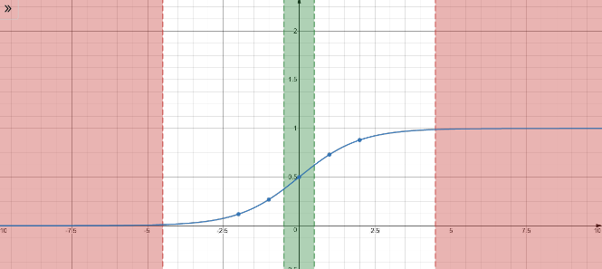
• When the parameters are too large - the activations become larger and larger (i.e tend to exist in the red region above), then your activations will saturate and become meaningless, with gradients approaching $0$.
• When the parameters are too small - the activations keep dropping layer after layer (i.e tend to exist in the green region above). At levels closer to zero the sigmoid activation function become more linear. Gradually the non-linearity is lost with derivatives of constants being $0$ and hence no benefit of multiple layers.

Summary Procedure of The Weight Initialization Algorithm

1. Evaluate $\theta^1$ using the input training patterns by applying Eqns $(18)$ and $(19)$ with $l =1$
2. The weights $w_{i\rightarrow j}^1$ are initialized by a random number generator with uniform distribution between $-\theta^1$ to $\theta^1$ or normal distribution $\mathcal N (0,(\theta_p^l)^2)$
3. Evaluate $a_{p,i}^2$ by feedforwarding the input patterns through the network using $w_{i\rightarrow j}^1$
4. For $l = 1,2,\dotsm,L-2$
   • Evaluate $\theta^1$ using the outputs of layer $l$, i.e $a_{p,i}^l$ and applying Eqns $(18)$ and $(19)$
   • The weights $w_{i\rightarrow j}^1$ are initialized by a random number generator with uniform distribution between $-\theta^l$ to $\theta^l$ or normal distribution $\mathcal N (0,(\theta_p^l)^2)$
   • Evaluate $a_{p,i}^{l+1}$ by feedforwarding the outputs of $a_{p,i}^{l}$ through the network using $w_{i\rightarrow j}^l$

5. After finding $a_{p,i}^{L-1}$ or $A^{L-1}$, we can find the last layer of weights $W^{L-1}$ by solving the following equation using a least-squares method, $$ \begin{align} \Vert A^{L-1}W^{L-1} - S \Vert_2 \tag{20} \end{align} $$

   • $S$ is a matrix, which has entries, $$ \begin{align} s_{i,j} = f^{-1}(t_{i,j}) \tag{21} \end{align} $$

   • where $t_{i,j}$ are the entries of target matrix $T$.

The weight initialization process is then completed. The linear least-squares problem shown in Eqn$(20)$ can be solved by QR factorization using Householder reflections [4].

In the case of an overdetermined system, QR factorization produces a solution that is the best approximation in a least-squares sense. In the case of an under-determined system, QR factorization computes the minimal-norm solution.

Conclusions

In general the proposed algorithm with uniform distributed weights performs better than the algorithm with normal distributed weights. The proposed algorithm is also applicable to networks with different activation functions.

It is worth noting that the time required for the initialization process is negligible when compared with training process.

References

1. A weight initialization method for improving training speed in feedforward neural network Jim Y.F. Yam, Tommy W.S. Chow (1998) [PDF]
2. Y.F. Yam, T.W.S. Chow, Determining initial weights of feedforward neural networks based on least-squares method, Neural Process. Lett. 2 (1995) 13-17.
3. Y.F. Yam, T.W.S. Chow, A new method in determining the initial weights of feedforward neural networks, Neurocomputing 16 (1997) 23-32.
4. G.H. Golub, C.F. Van Loan, Matrix Computations, The Johns Hopkins University Press, Baltimore, MD, 1989