Factorization Machines

Jefkine, 27 March 2017

Introduction

Factorization machines were first introduced by Steffen Rendle [1] in 2010. The idea behind FMs is to model interactions between features (explanatory variables) using factorized parameters. The FM model has the ability to the estimate all interactions between features even with extreme sparsity of data.

FMs are generic in the sense that they can mimic many different factorization models just by feature engineering. For this reason FMs combine the high-prediction accuracy of factorization models with the flexibility of feature engineering.

From Polynomial Regression to Factorization Machines

In order for a recommender system to make predictions it relies on available data generated from recording of significant user events. These are records of transactions which indicate strong interest and intent for instance: downloads, purchases, ratings.

For a movie review system which records as transaction data; what rating $r \in \lbrace 1,2,3,4,5 \rbrace$ is given to a movie (item) $i \in I$ by a user $u \in U$ at a certain time of rating $t \in \mathbb{R}$, the resulting dataset could be depicted as follows:

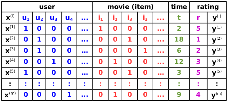
If we model this as a regression problem, the data used for prediction is represented by a design matrix $X \in \mathbb{R}^{m \times n}$ consisting of a total of $m$ observations each made up of real valued feature vector $\mathbf{x} \in \mathbb{R}^n$. A feature vector from the above dataset could be represented as:

$\begin{align} (u,i,t) \rightarrow \mathbf{x} = (\underbrace{0,..,0,1,0,...,0}_{|U|},\underbrace{0,..,0,1,0,...,0}_{|I|},\underbrace{0,..,0,1,0,...,0}_{|T|}) \end{align} \$

where $n = \vert U \vert + \vert I \vert + \vert T \vert$ i.e $\mathbf{x} \in \mathbb{R}^n$ is also represented as $\mathbf{x} \in \mathbb{R}^{\vert U \vert + \vert I \vert + \vert T \vert}$

This results in a supervised setting where the training dataset is organised in the form $D = \lbrace (x^{(1)}, y^{(1)}), (x^{(2)}, y^{(2)}),...(x^{(m)}, y^{(m)})\rbrace$. Our task is to estimate a function $\hat{y}\left( \mathbf{x} \right) : \mathbb{R}^n \ \rightarrow \mathbb{R}$ which when provided with $i^{\text{th}}$ row $x^{i} \in \mathbb{R}^n$ as the input to can correctly predict the corresponding target $y^{i} \in \mathbb{R}$.

Using linear regression as our model function we have the following:

$\begin{align} \hat{y}(\textbf{x}) = w_{0} + \sum_{i=1}^{n} w_{i} x_{i} \tag {1} \end{align} \$

Parameters to be learned from the training data

• $w_{0} \in \mathbb{R}$ is the global bias
• $\textbf{w} \in \mathbb{R}^n$ are the weights for feature vector $\textbf{x}_i \; \forall i$

With three categorical variables: user $u$, movie (item) $i$, and time $t$, applying linear regression model to this data leads to:

$\begin{align} \hat{y}(\textbf{x}) = w_{0} + w_{u} + w_{i} + w_{t} \tag {2} \end{align} \$

This model works well and among others has the following advantages:

• Can be computed in linear time $O(n)$
• Learning $\textbf{w}$ can be cast as a convex optimization problem

The major drawback with this model is that it does not handle feature interactions. The three categorical variables are learned or weighted individually. We cannot therefore capture interactions such as which user likes or dislikes which movie (item) based on the rating they give.

To capture this interaction, we could introduce a weight that combines both user $u$ and movie (item) $i$ interaction i.e $w_{ui}$.

An order $2$ polynomial has the ability to learn a weight $w_{ij}$ for each feature combination. The resulting model is shown below:

$\begin{align} \hat{y}(\textbf{x}) = w_{0} + \sum_{i=1}^{n} w_{i} x_{i} + \sum_{i=1}^n \sum_{j=i+1}^n x_{i} x_{j} w_{ij} \tag {3} \end{align} \$

Parameters to be learned from the training data

• $w_{0} \in \mathbb{R}$ is the global bias
• $\textbf{w} \in \mathbb{R}^n$ are the weights for feature vector $\textbf{x}_i \; \forall i$
• $\textbf{W} \in \mathbb{R}^{n \times n}$ is the weight matrix for feature vector combination $\textbf{x}_i \textbf{x}_j \; \forall i \; \forall j$

With three categorical variables: user $u$, movie (item) $i$, and time $t$, applying order $2$ polynomial regression model to this data leads to:

$\begin{align} \hat{y}(\textbf{x}) = w_{0} + w_{u} + w_{i} + w_{t} + w_{ui} + w_{ut} + w_{ti} \tag {4} \end{align} \$

This model is an improvement over our previous model and among others has the following advantages:

• Can capture feature interactions at least for two features at a time
• Learning $\textbf{w}$ and $\textbf{W}$ can be cast as a convex optimization problem

Even with these notable improvements over the previous model, we still are faced with some challenges including the fact that we have now ended up with a $O(n^2)$ complexity which means that to train the model we now require more time and memory.

A key point to note is that in most cases, datasets from recommendation systems are mostly sparse and this will adversely affect the ability to learn $\textbf{W}$ as it depends on the feature interactions being explicitly recorded in the available dataset. From the sparse dataset, we cannot obtain enough samples of the feature interactions needed to learn $w_{ij}$.

The standard polynomial regression model suffers from the fact that feature interactions have to be modeled by an independent parameter $w_{ij}$. Factorization machines on the other hand ensure that all interactions between pairs of features are modeled using factorized interaction parameters.

The FM model of order $d = 2$ is defined as follows:

$\begin{align} \hat{y}(\textbf{x}) = w_{0} + \sum_{i=1}^{n} w_{i} x_{i} + \sum_{i=1}^{n} \sum_{j=i+1}^n \langle \textbf{v}_i , \textbf{v}_{j} \rangle x_i x_{j} \tag {5} \end{align} \$

$\langle \cdot \;,\cdot \rangle$ is the dot product of two feature vectors of size $k$:

$\begin{align} \langle \textbf{v}_i , \textbf{v}_{j} \rangle = \sum_{f=1}^k v_{i,f} v_{j,f} \tag {6} \end{align} \$

This means that Eq. $5$ can be written as:

$\begin{align} \hat{y}(\textbf{x}) = w_{0} + \sum_{i=1}^{n} w_{i} x_{i} + \sum_{i=1}^{n} \sum_{j=i+1}^n x_i x_{j} \sum_{f=1}^k v_{i,f} v_{j,f} \tag {7} \end{align} \$

Parameters to be learned from the training data

• $w_{0} \in \mathbb{R}$ is the global bias
• $\textbf{w} \in \mathbb{R}^n$ are the weights for feature vector $\textbf{x}_i \; \forall i$
• $\textbf{V} \in \mathbb{R}^{n \times k}$ is the weight matrix for feature vector combination $\textbf{v}_i \textbf{v}_j \; \forall i \; \forall j$

With three categorical variables: user $u$, movie (item) $i$, and time $t$, applying factorization machines model to this data leads to:

$\begin{align} \hat{y}(\textbf{x}) = w_{0} + w_{u} + w_{i} + w_{t} + \langle \textbf{v}_u , \textbf{v}_{i} \rangle + \langle \textbf{v}_u , \textbf{v}_{t} \rangle + \langle \textbf{v}_t , \textbf{v}_{i} \rangle \tag {8} \end{align} \$

The FM model replaces feature combination weights $w_{ij}$ with factorized interaction parameters between pairs such that $w_{ij} \approx \langle \textbf{v}_{i}, \textbf{v}_{j} \rangle = \sum_{f=1}^k v_{i,f} v_{j,f}$.

Any positive semi-definite matrix $\textbf{W} \in \mathbb{R}^{n \times n}$ can be decomposed into $\textbf{VV}^\top$ (e.g., Cholesky Decomposition). The FM model can express any pairwise interaction matrix $\textbf{W} = \textbf{VV}^\top$ provided that the $k$ chosen is reasonably large enough. $\textbf{V} \in \mathbb{R}^k$ where $k \ll n$ is a hyper-parameter that defines the rank of the factorization.

The problem of sparsity nonetheless implies that the $k$ chosen should be small as there is not enough data to estimate complex interactions $\textbf{W}$. Unlike in polynomial regression we cannot use the full matrix $\textbf{W}$ to model interactions.

FMs learn $\textbf{W} \in \mathbb{R}^{n \times n}$ in factorized form hence the number of parameters to be estimated is reduced from $n^2$ to $n \times k$ since $k \ll n$. This reduces overfitting and produces improved interaction matrices leading to better prediction under sparsity.

The FM model equation in Eq. $7$ now requires $O(kn^2)$ because all pairwise interactions have to be computed. This is an increase over the $O(n^2)$ required in the polynomial regression implementation in Eq. $3$.

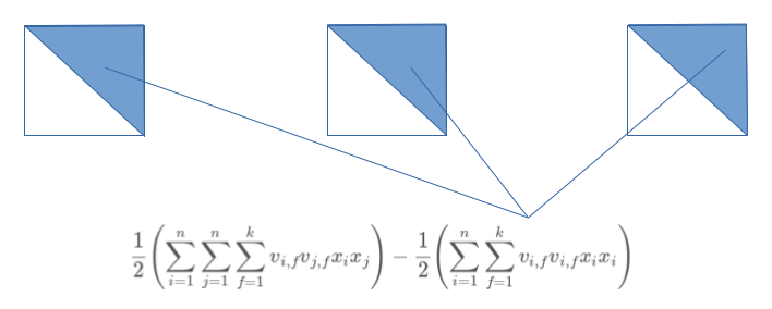
With some reformulation however, we can reduce the complexity from $O(kn^2)$ to a linear time complexity $O(kn)$ as shown below:

$$\begin{align} & \sum_{i=1}^n \sum_{j=i+1}^n \langle \textbf{v}_i , \textbf{v}_{j} \rangle x_{i} x_{j} \\ &= \frac{1}{2} \sum_{i=1}^n \sum_{j=1}^n \langle \textbf{v}_i , \textbf{v}_{j} \rangle x_{i} x_{j} - \frac{1}{2} \sum_{i=1}^n \langle \textbf{v}_i , \textbf{v}_{i} \rangle x_{i} x_{i} \tag {A} \\ &= \overbrace{ \frac{1}{2}\left(\sum_{i=1}^n \sum_{j=1}^n \sum_{f=1}^k v_{i,f} v_{j,f} x_{i} x_{j} \right) }^{\bigstar} - \overbrace{\frac{1}{2}\left( \sum_{i=1}^n \sum_{f=1}^k v_{i,f} v_{i,f} x_{i} x_{i} \right) }^{\bigstar \bigstar} \tag {B} \\ &= \frac{1}{2}\left(\sum_{i=1}^n \sum_{j=1}^n \sum_{f=1}^k v_{i,f} v_{j,f} x_{i} x_{j} - \sum_{i=1}^n \sum_{f=1}^k v_{i,f} v_{i,f} x_{i} x_{i} \right) \\ &= \frac{1}{2} \sum_{f=1}^{k} \left( \left(\sum_{i=1}^n v_{i,f}x_{i} \right) \left( \sum_{j=1}^n v_{j,f}x_{j} \right) - \sum_{i=1}^{n} v_{i,f}^2 x_{i}^2 \right) \\ &= \frac{1}{2} \sum_{f=1}^{k} \left( \left( \sum_{i}^{n} v_{i,f}x_{i} \right)^2 - \sum_{i=1}^{n} v_{i,f}^2 x_{i}^2 \right) \tag {9} \end{align} \ $$

The positive semi-definite matrix $\mathbf{W} = \mathbf{VV}^\top$ which contains the weights of pairwise feature interactions is symmetric. With symmetry, summing over different pairs is the same as summing over all pairs minus the self-interactions (divided by two). This is the reason why the value $\frac{1}{2}$ is introduced as from Eq. $A$ and beyond.

Let us use some images to expound on this equations even further. For our purposes we will use a $3 \; \text{by} \; 3$ symmetric matrix from which we are expecting to end up with $\sum_{i=1}^n \sum_{j=i+1}^n \langle \textbf{v}_i , \textbf{v}_{j} \rangle x_{i} x_{j}$ as follows:

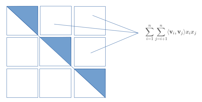
The first part of the Eq. $B$ marked $\bigstar$ represents a half of the $3 \; \text{by} \; 3$ symmetric matrix as shown below:

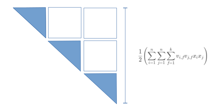
To end up with our intended summation $\sum_{i=1}^n \sum_{j=i+1}^n \langle \textbf{v}_i , \textbf{v}_{j} \rangle x_{i} x_{j}$, we will have to reduce the summation shown above with the second part of Eq. $B$ marked $\bigstar \bigstar$ as follows:

Substistuting Eq. $9$ in Eq. $7$ we end up with an equation of the form:

$\begin{align} \hat{y}(\textbf{x}) = w_{0} + \sum_{i=1}^{n} w_{i} x_{i} + \frac{1}{2} \sum_{f=1}^{k} \left( \left( \sum_{i}^{n} v_{i,f}x_{i} \right)^2 - \sum_{i=1}^{n} v_{i,f}^2 x_{i}^2 \right) \tag {10} \end{align} \$

Eq. $10$ now has linear complexity in both $k$ and $n$. The computation complexity here is $O(kn)$.

For real world problems most of the elements $x_i$ in the feature vector $\mathbf{x}$ are zeros. With this in mind lets go ahead and define some two quantities here:

• $N_z(\mathbf{x})$ - the number of non-zero elements in feature vector $\mathbf{x}$
• $N_z(\mathbf{X})$ - the average number of none-zero elements of all vectors $\mathbf{x} \in D$ (average for the whole dataset $D$ or the number of non-zero elements in the design matrix $\mathbf{X}$)

From our previous equations it is easy to see that the numerous zero values in the feature vectors will only leave us with $N_z(\mathbf{X})$ non zero values to work with in the summation (sums over $i$) on Eq. $10$ where $N_z(\mathbf{X}) \ll n$. This means that our complexity will drop down even further from $O(kn)$ to $O(kN_{z}( \mathbf{X}))$.

This can be seen as a much needed improvement over polynomial regression with the computation complexity of $O(N_{z}( \mathbf{X})^2)$.

Learning Factorization Machines

FMs have a closed model equation which can be computed in linear time. Three learning methods prposed in [2] are stochastic gradient descent(SGD), alternating least squares (ALS) and Markov Chain Monte Carlo (MCMC) inference.

The model parameters to be learned are $(w_0, \mathbf{w},$ and $\mathbf{V} )$. The loss function chosen will depend on the task at hand. For example:

• For regression, we use least square loss: $l(\hat{y}(\textbf{x}) , y) = (\hat{y}(\textbf{x}) - y)^2$
• For binary classification, we use logit or hinge loss: $l(\hat{y}(\textbf{x}) , y) = - \ln \sigma(\hat{y}(\textbf{x}){y})$ where $\sigma$ is the sigmoid/logistic function and $y \in {-1,1}$.

FMs are prone to overfitting and for this reason $L2$ regularization is applied. Finally, the gradients of the model equation for FMs can be depicted as follows:

$$\begin{align} \frac{\partial}{\partial\theta}\hat{y}(\textbf{x}) = \begin{cases} 1, & \text{if $\theta$ is $w_0$} \\ x_i, & \text{if $\theta$ is $w_i$} \\ x_i\sum_{j=1}^{n} v_{j,f}x_j - v_{i,f}x_{i}^2 & \text{if $\theta$ is $v_{i,f}$} \end{cases} \end{align}$$

Notice that the sum $\sum_{j=1}^{n} v_{j,f}x_j$ is independent of $i$ and thus can be precomputed. Each gradient can be computed in constant time $O(1)$ and all parameter updates for a case $(x,y)$ can be done in $O(kn)$ or $O(kN_z(\mathbf{x}))$ under sparsity.

For a total of $i$ iterations all the proposed learning algorithms can be said to have a runtime of $O(kN_z(\mathbf{X})i)$.

Conclusions

FMs also feature some notable improvements over other models including

• FMs model equation can be computed in linear time leading to fast computation of the model
• FM models can work with any real valued feature vector as input unlike other models that work with restricted input data
• FMs allow for parameter estimation even under very sparse data
• Factorization of parameters allows for estimation of higher order interaction effects even if no observations for the interactions are available

References

1. A Factorization Machines by Steffen Rendle - In: Data Mining (ICDM), 2010 IEEE 10th International Conference on. (2010) 995–1000 [PDF]
2. Factorization machines with libfm S Rendle ACM Transactions on Intelligent Systems and Technology (TIST) 3 (3), 57 (2012) [PDF]